
To provide some background information for my N-link pendulum project, I’ve broken the methodology for solving the equations of motion (EOM) for a simple double pendulum into a separate post. I’ll explain to the best of my abilities!
The pendulum that we are solving for is composed of two masses, m1 and m2, suspended from each other by strings of length l1 and l2. Their positions relative to 0 is represented by theta1 and theta2. The entire pendulum is supported by point 0, which is a frictionless, massless point. The whole thing is a pain to create digitally, so I drew the setup below:

This will be a pretty long post, so scroll to the bottom for the cool graphs!
We’ll find the equations of motion in Polar coordinates, since it means that we only need two equations instead of four. (The two being 
By doing basic trig, we can find the EOM of the masses using time derivatives of the unit vectors. In this case, 

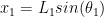
Position:


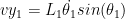
Velocity:


Acceleration:


We know that 
The sum of forces is:


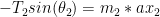

Note at ax1, ay1, etc. are the same as the acceleration equations we previously found.
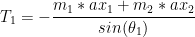
Because tension is a reactionary force, we’ll solve for T1 and T2 in order to isolate equations for
Solving for T1:


Setting the two equations equal to each other:
![-cos(\theta_1)[m_1 * ax_1 + m_2 * ax_2] = sin(\theta_1)[m_1 * ay_1 + m_2 * ay_2 + m_1g + m_2g]](http://s0.wp.com/latex.php?latex=-cos%28%5Ctheta_1%29%5Bm_1+%2A+ax_1+%2B+m_2+%2A+ax_2%5D+%3D+sin%28%5Ctheta_1%29%5Bm_1+%2A+ay_1+%2B+m_2+%2A+ay_2+%2B+m_1g+%2B+m_2g%5D&bg=ffffff&fg=000&s=0&c=20201002)
Now for T2:
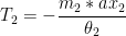
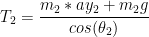
Setting the two equal:
![cos(\theta_2)m_2 * ax_2 = sin(\theta_2)[m_2 * ay_2 + m_2g]](http://s0.wp.com/latex.php?latex=cos%28%5Ctheta_2%29m_2+%2A+ax_2+%3D+sin%28%5Ctheta_2%29%5Bm_2+%2A+ay_2+%2B+m_2g%5D&bg=ffffff&fg=000&s=0&c=20201002)
Now we have two equations and two unknowns! We can solve for 

I did all the wrong math so you don’t have to! 😀
UNTIL I REALIZED that I had dropped a negative sign. Throw it into Matlab using the syms function and have it spit out the correct equations. Which, if you were curious, look like this:
t1dd = -(L1*M2*sin(2*t1 - 2*t2)*t1d^2 + 2*L2*M2*sin(t1 - t2)*t2d^2 + M2*g*sin(t1 - 2*t2) + 2*M1*g*sin(t1) + M2*g*sin(t1))/(L1*(2*M1 + M2 - M2*cos(2*t1 - 2*t2)));
t2dd = (M1*g*sin(2*t1 - t2) + M2*g*sin(2*t1 - t2) - M1*g*sin(t2) - M2*g*sin(t2) + L2*M2*t2d^2*sin(2*t1 - 2*t2) + 2*L1*M1*t1d^2*sin(t1 - t2) + 2*L1*M2*t1d^2*sin(t1 - t2))/(L2*(2*M1 + M2 - M2*cos(2*t1 - 2*t2)));
(terrifying).
Using all this information, you can put the equations into Matlab’s ODE45 to plot the motion of the simple pendulum!

The cartesian displacement of the two masses. Note how M1 is circular (as expected), while M2 moves in a bowl like path because its trajectory is dependent on M1.

The energy graph shows that kinetic energy (KE) added to potential energy (PE) results in a flat total energy (TE). Energy is conserved, yay!

The position/velocity/acceleration plot for M1 is quite turbulent, because M1 has more forces acting on it than M2.

M2’s motion is as expected.

Finally, we see that the tension forces on M1 and M2 add to 0. Because Newton’s third law!
Whew, that was quite a ride. Cool, innit?
-Sophie
Much appreciated!
Glad I could help!